Recovering packets from overlapping radio signals
Following MOSAIC's receiver from a decoded packet to a reconstructed waveform, and separating the UHF measurements from the remaining HF questions.
On this page
When two transmitters overlap, a receiver gets a mixture of their signals. If it can decode one complete packet, it gains something useful beyond the text of the message: it knows what that transmitter was trying to send. Given the modulation rules and a sufficiently good estimate of the received signal, it can reconstruct that packet’s waveform, subtract it from the recording and try decoding what remains.
That is the part of MOSAIC I want to explain here. The August work includes a recorded three-radio UHF browser exchange on the 14th and retained mixed-rate captures on the 15th. The public source release and whitepaper make it possible to follow the receiver through those steps, including the places where a plausible-looking candidate must be rejected before it changes the recording.
Knowing the bits is only part of knowing the signal
MOSAIC sends four coded bits per symbol by choosing one tone from sixteen candidates. An access signature determines how those candidate tones are placed in the frequency grid over time. The receiver can search a finite catalogue of signatures, acquire possible packets and rank them by the observed acquisition score.
A catalogue entry doesn’t mean that transmitter was active. It gives the receiver a hypothesis to try. The ordinary packet decoder still has to recover a payload that passes its CRC before the cancellation process is allowed to use it.
The cancellation step can be written quite compactly:
new residual = old residual - fitted packet waveformThe fitting is where much of the work sits. Transmitters don’t arrive with a common oscillator or an exact shared start time. The decoded bits tell us which waveform to construct, but its timing, frequency offset, drift, gain and phase still have to match what reached the receiver. Subtracting the right message with the wrong phase or amplitude can leave a poor residual.
In the released implementation, the original samples are retained separately from the residual. Cancellation records the previous segment in a ledger, along with the fitted parameters, so that subtraction can be reversed. The search and number of cancellation generations are bounded. Passing the CRC is a gate into this process, not a guarantee of a perfect fit or a promise that every other packet will become decodable.
The live modem also has a quicker route through the same problem. It first tries the catalogue signatures independently, which can recover packets without needing a full cancellation search. When that leaves an incomplete set, it can peel decoded signals from the residual and continue looking.
What the radios demonstrated
The published measurements distinguish several kinds of evidence. An early retained multi-transmitter capture used a bladeRF x115 and a USRP B210 as physically separate transmitters, with a HackRF One receiving both. Later captures put more logical station identities through those two transmit chains. Twelve recovered identities in that arrangement means twelve logical stations, not twelve independent radios.
The mixed-rate experiment is useful because it gives the receiver several packet timings and rates to deal with in the same passband. Here are the reported results for two retained captures:
| Waveforms carried at 431.200 MHz | CRC-valid profiles recovered | Declared time with two or more users overlapping |
|---|---|---|
| UHF Basic, Fast and Turbo | 3 of 3 | 53.4% |
| HF Basic, Chat and Fast | 3 of 3 | 51.3% |
Both captures used a 431.200 MHz UHF carrier, with the second carrying the slower HF-family waveforms. That let the same radio arrangement exercise both profile families, including their different symbol timings and packet lengths.
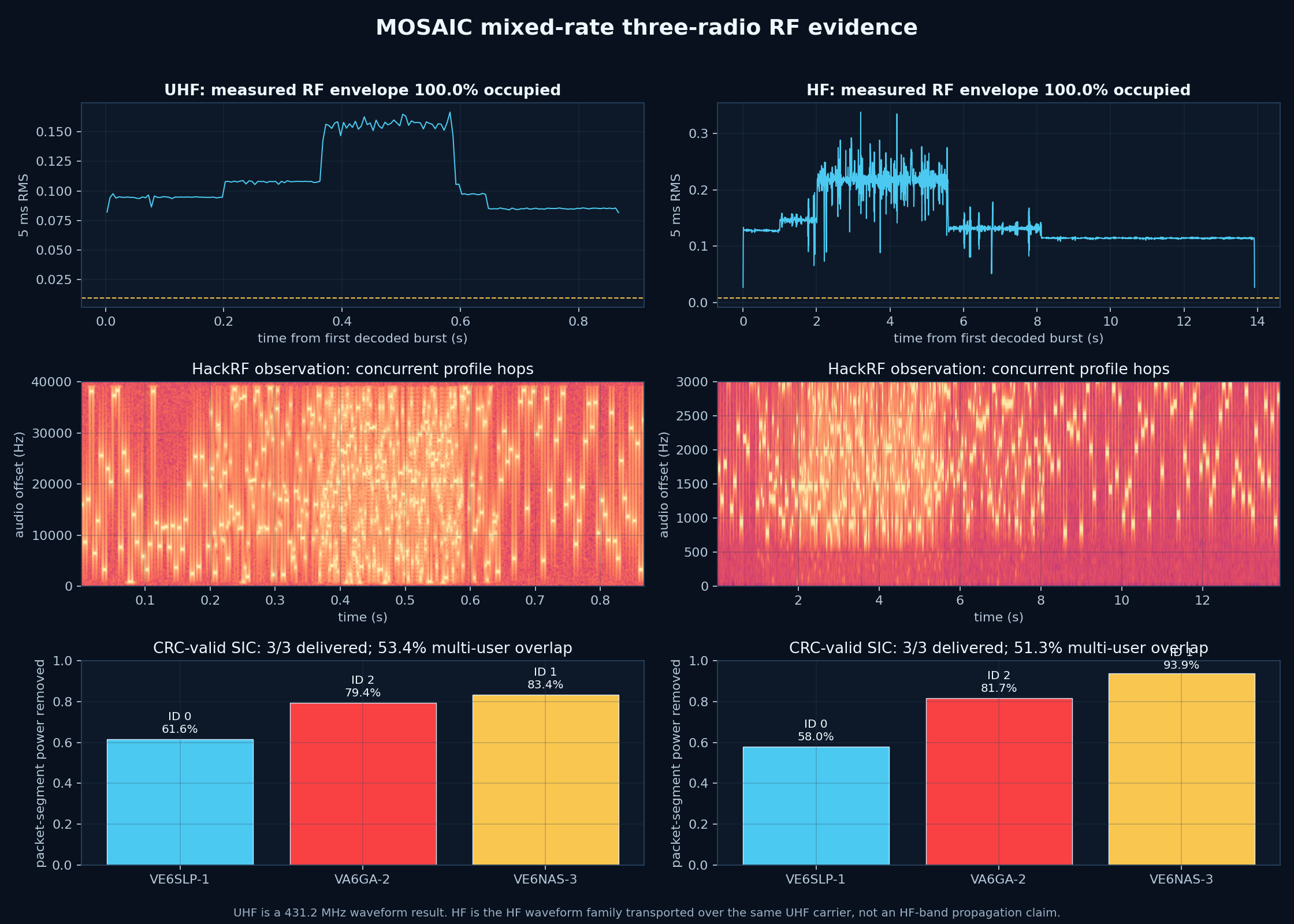
Published August RF evidence, reproduced from the MOSAIC project. Open the figure for the full-size axes and labels. Both columns use 431.200 MHz; “HF” labels the waveform family in the right column.
The upper panels measure the envelope in five-millisecond RMS blocks, from the first decoded packet’s start to the last one’s end. Within that window, every block exceeds the threshold derived from the guard and active portions of the capture, giving the reported 100% occupancy. The middle panels show changing tone occupancy, and the lower ones show how much packet-segment power was removed by cancellation. That power reduction is a separate measurement from the three CRC-valid packets recovered in each capture. Together they describe these particular UHF experiments; delivery rates over longer runs, sustainable network capacity and propagation on an HF band need their own measurements.
The slower waveform leaves another experiment to do
The basic HF profile uses 80-millisecond symbols and 12.5 Hz tone spacing. The basic UHF profile uses five-millisecond symbols and 200 Hz spacing. In both cases, the product of symbol duration and tone spacing is one. With four coded bits per symbol, those settings give 50 and 800 coded bits per second respectively, before accounting for error correction, headers, preambles and the other costs between a waveform and delivered text.
The slower timing is only part of working on HF. Fading and multipath can change a signal while the receiver is trying to estimate and subtract it, which is why the public work includes separate software channel simulations and additional fitting machinery. Shared-channel operation through an ionospheric HF path remains to be demonstrated.